Gallery
UFEM
Spectral Difference Method (SDM)
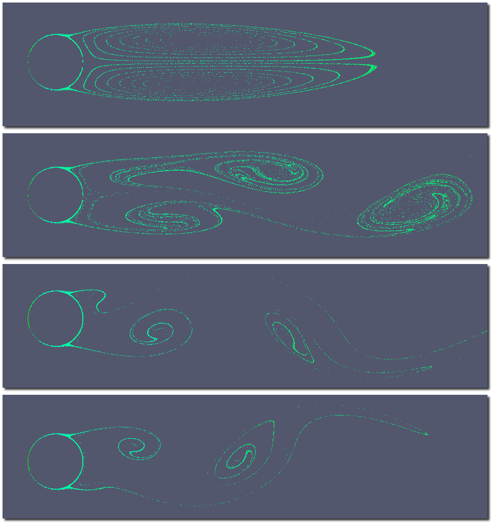
Inviscid flow past cylinder, Mach 0.38

Simulation of 2D inviscid flow past cylinder with Mach=0.38.
Euler equations are solved with a 3rd order Spectral Difference method on a 1024-element quadrangular P2-mesh.
Time integration is done with Backward Euler, solved by a non-linear LU-SGS iterative solver.
High-order visualization is done with Gmsh.
Inviscid flow over NACA-0012 airfoil, Mach 0.08, Attack angle 6.7°
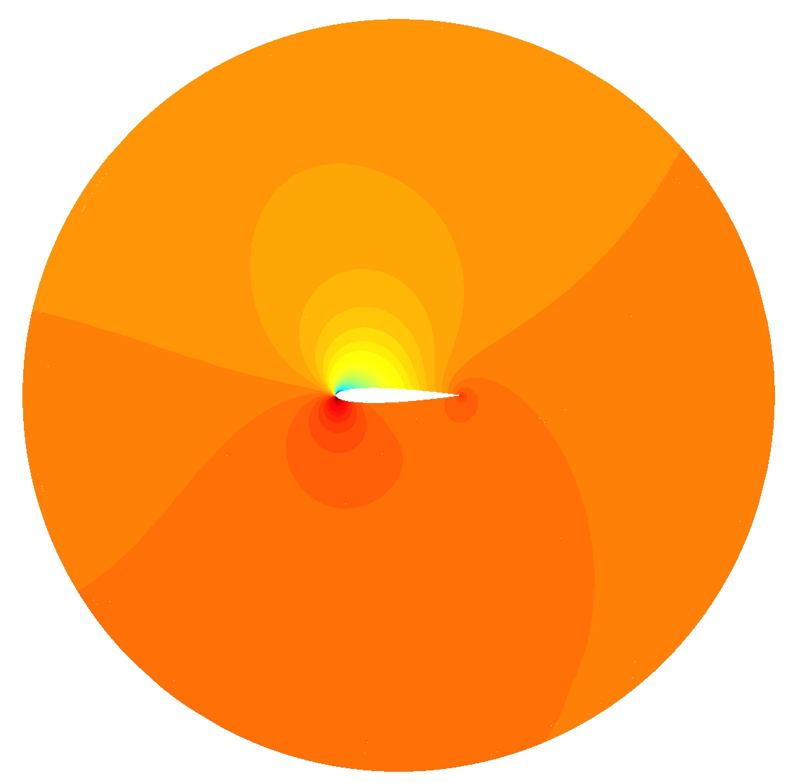
Simulation of 2D inviscid flow past NACA-0012 airfoil with Mach=0.08, angle of attack 6.7°
Euler equations are solved with a 3rd order Spectral Difference method
on a 6,666-element unstructured quadrangular mesh.
High-order visualization is done with Gmsh.
Inviscid flow past wedge, Mach 0.38
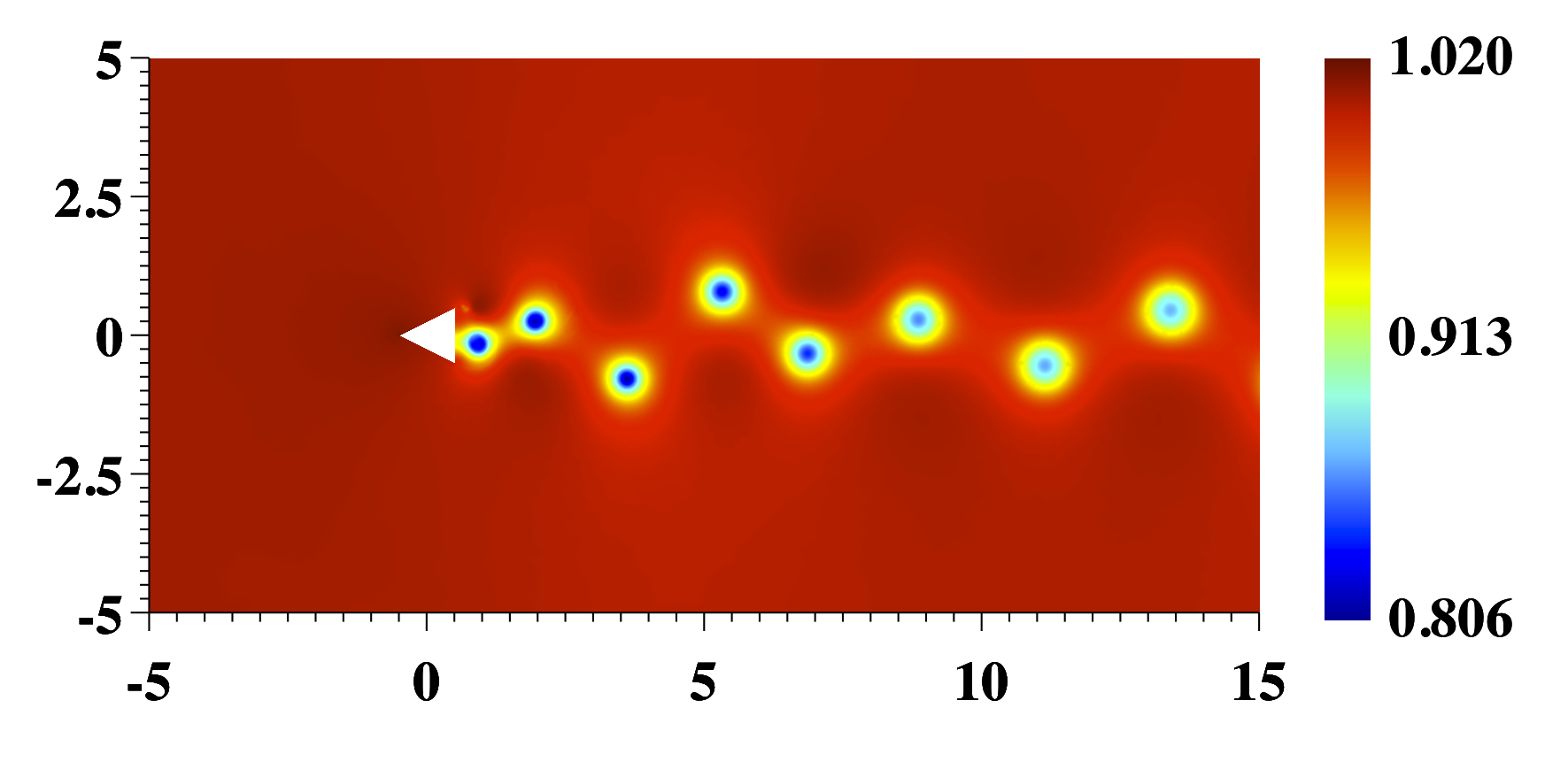
Simulation of 2D inviscid flow past triangular wedge with Mach=0.2.
Vortex shedding occurs due to numerical viscosity at the sharp trailing edges of the wedge.
Disclaimer: This is of course not a physical solution.
Euler equations are solved with a 4th order Spectral Difference method on a 11,686-element quadrangular mesh.
Time integration is done with a SD-optimized Explicit Runge-Kutta (18,4) method.
High-order visualization is done with Gmsh.
Acoustic pulse with vortex
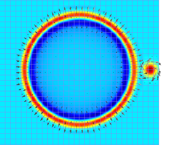
Simulation of an acoustic pulse and a vortex, in a mean-flow with Mach=0.5. This is a benchmark case to test the accuracy and outflow-boundary condition for the linearized Euler equations.
Linearized Euler equations (LEE) are solved with a 4th order Spectral Difference method on a 50x50 Cartesian mesh.
Time integration is done with Explicit Runge-Kutta (4,4) in low-storage form.
High-order visualization is done with Gmsh.
Mach-cone, Mach 1.5
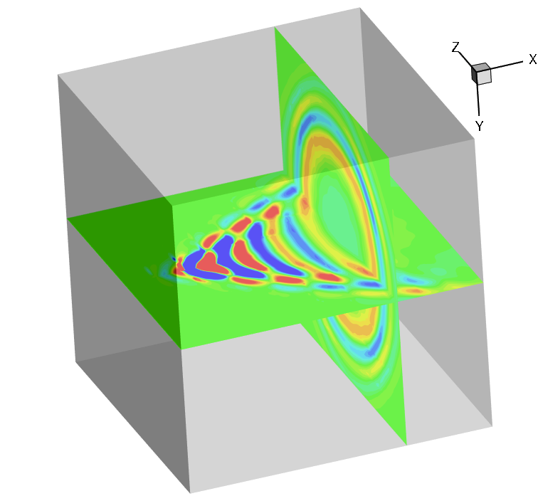
Simulation of 3D monopole source term in a background flow with Mach=1.5
Because of the supersonic background flow, the typical mach-cone becomes visible.
The Linearized Euler equations (LEE) are solved with a 5th order Spectral Difference method on a 10x10x10-element hexahedral mesh.
Time integration is done with a low-storage Explicit Runge-Kutta (3,3) method.
High-order visualization is done by interpolating the high-order polynomial solution from the 10x10x10-element mesh to a
fine 100x100x100-element mesh and exporting to Tecplot.
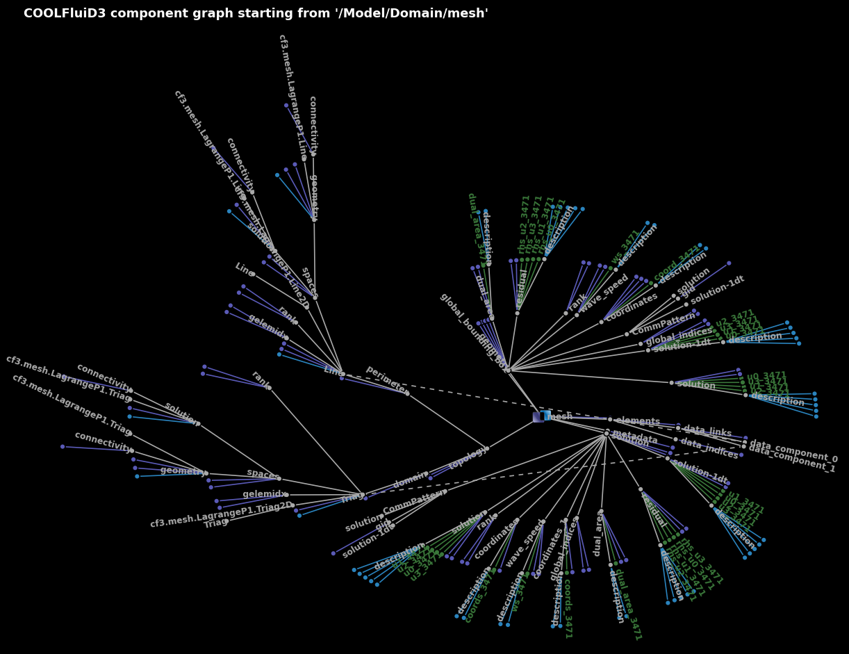
Coolfluid Kernel API
Component structure of a typical 2D mesh
Detailed information of a Component
